A well-architected data pipeline is not just about writing good transformation logic — it is equally about where that logic runs and how the data is organized at each stage of its journey. Two foundational design patterns address these concerns: physical environment separation and layer separation. Together, they give data engineering teams the isolation, safety, and clarity needed to develop, test, and operate pipelines confidently at scale.
Part 1: Physical Environment Separation
What Is Physical Environment Separation?
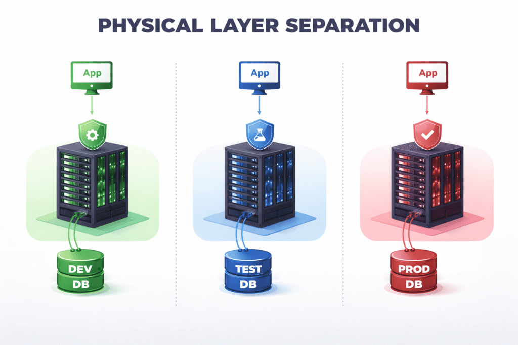
Physical environment separation means running your pipeline infrastructure across entirely distinct, isolated computing resources — not just different configurations on the same cluster or server. The idea is straightforward: code and data that belong to development should never share resources with production. Mistakes made in development stay contained, and production remains stable and untouched.
How to Implement It
The approach differs slightly depending on your infrastructure of choice.
On cloud-native platforms like Databricks or AWS, the recommended approach is to use separate workspaces, accounts, or shards. On Databricks, this means provisioning a distinct workspace per environment. On AWS, this typically means using separate AWS accounts — a well-established pattern that AWS itself recommends for enterprise workloads — or at minimum, separate Glue databases, S3 buckets, and IAM boundaries scoped to each environment.
On self-managed database systems like PostgreSQL, physical separation means running distinct server instances. A dev team should connect to a different host than the test and production teams. Relying on schema-level separation (for example, a dev_schema vs a prod_schema on the same Postgres instance) is not sufficient — a misconfigured connection string or a runaway DELETE statement could affect both environments simultaneously.
The Three Standard Environments
A typical setup uses three environments:
Development (dev) is where engineers do their initial work. They experiment, write new transformations, debug logic, and iterate freely. Because this environment is isolated, a broken job or a dropped table causes no harm beyond slowing down the engineer themselves.
Test (test) is a close mirror of production. It uses the same infrastructure size, the same configuration, and ideally the same data shapes and volumes. The purpose of the test environment is to validate that code which worked in dev will also behave correctly under conditions that resemble the real world. If test diverges too far from prod — for example, by using a smaller cluster or a much smaller dataset — tests lose their value as a reliability signal.
Production (prod) is where real business workloads run, serving dashboards, downstream teams, and external consumers. It is treated as sacred: no one runs ad-hoc queries against production tables, no one manually triggers jobs outside of the CI/CD system, and no schema changes happen without a reviewed and merged pull request.
Why Physical Separation Matters
Data isolation and security. Production data often contains sensitive information, including personally identifiable information (PII) such as names, email addresses, or payment details. Physical separation makes it straightforward to mask or anonymize this data before it is made available in dev and test environments. Developers can work with realistic data shapes without ever touching real customer data.
Enforcing code discipline. When only the CI/CD pipeline has the credentials and permissions to deploy and trigger jobs in production, you get a powerful guarantee: only reviewed, checked-in code ever runs on prod. There are no mystery jobs, no one-off scripts that a teammate ran last Tuesday, and no “I’ll just fix it quickly in production” moments. Every change has a traceable commit behind it.
Handling production hotfixes safely. Some teams worry that strict environment separation makes emergency fixes too slow. In practice, the opposite is true. Even in a hotfix scenario, the process is well-defined: raise a hotfix PR, get a quick review, merge it, and let the CI/CD pipeline deploy it. This takes minutes and still produces an auditable trail. It is far safer than giving engineers direct production access and hoping they don’t make things worse under pressure.
Preventing accidental cross-contamination. Without physical separation, it is surprisingly easy for a development job to accidentally read from or write to a production table, especially when pipelines grow large and connection strings are managed inconsistently. Hard boundaries at the infrastructure level make this class of mistake impossible.
Part 2: Layer Separation
What Is Layer Separation?
Layer separation is the practice of organizing data into distinct logical zones — typically called layers — within a single physical environment. While physical separation answers the question “which environment is this?”, layer separation answers the question “what stage of processing is this data at?” Each layer has a clear purpose, and data flows through them in one direction: from raw ingestion toward business-ready outputs.
The Four Standard Layers
A well-structured data pipeline typically organizes data into four layers: raw, stage, bus, and serv.
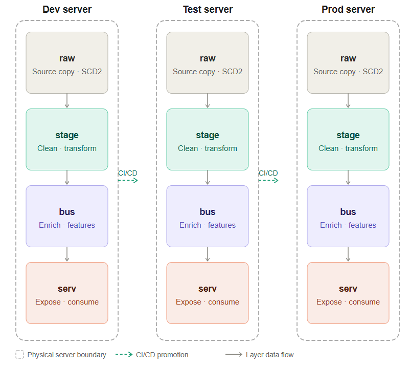
Raw Layer
The raw layer is the landing zone for data exactly as it arrived from the source system. No transformations, no filtering, no business logic — just a faithful copy of what was ingested.
A common pattern here is to apply SCD Type 2 (Slowly Changing Dimension Type 2) logic and stamp each record with a processing_ts (processing timestamp). This means that every version of a record is preserved over time, giving you a complete historical ledger of what the source system sent and when.
The raw layer is invaluable for debugging. When a data issue surfaces weeks or months later — a duplicated record, an unexpected null, a source system that quietly changed its schema — the raw layer lets you go back to the original data and trace exactly what happened. Without it, the investigation would be much harder because downstream transformations have already altered the data.
Stage Layer
The stage layer is where data begins to take on the shape your business needs. Raw data is cleaned, standardized, and transformed here.
Typical operations at this layer include renaming and recasting columns to match agreed-upon naming conventions, handling nulls and data quality issues, and applying deduplication logic. Crucially, the stage layer is also where you aggregate to the required grain — that is, you decide whether you need hourly, daily, or monthly records, and collapse the raw data accordingly. Choosing the right grain at this stage prevents expensive re-aggregation work downstream and ensures that all subsequent layers are working with consistently sized records.
Think of the stage layer as the point where raw signals are turned into clean, well-formed facts that are ready to be reasoned about.
Business (Bus) Layer
The bus layer holds enriched, intermediate data that is not yet ready for external consumption but is more valuable than what the stage layer produced. This is where most of the complex business logic lives.
Several types of transformations are common at this layer:
Enrichment involves joining stage data with reference or lookup tables — sometimes called legend data — to add context. For example, a raw event might contain a product_id, and the bus layer joins it with a product dimension table to add the product name, category, and price tier.
Feature engineering for machine learning pipelines also belongs here. If your data platform supports ML workloads, the bus layer is the natural place to compute derived features — rolling averages, lag features, ratios — that will feed into model training or inference pipelines.
Intermediate aggregations that serve multiple downstream consumers can also live here, avoiding the need to compute the same expensive rollup in several different places.
The bus layer acts as a reusable library of well-processed data assets that multiple downstream consumers — dashboards, other teams, ML pipelines — can draw from independently.
Serve (Serv) Layer
The serve layer is the outermost layer, and the only one that external consumers interact with directly. This is where data is packaged for delivery.
If you maintain a business intelligence dashboard, the final aggregated table that powers it lives in the serve layer. If another team has requested access to a particular dataset, the version of that dataset that is shared with them is in the serve layer. If you expose data via an API, the tables backing that API live here.
The serve layer is deliberately kept clean and minimal. It contains only what consumers need, modeled in the way they need it. Internal intermediate tables, experimental features, and half-processed datasets do not belong here. The serve layer is a contract with your consumers: this data is production-quality, well-documented, and stable.
Why the Layered Flow Matters
The flow raw → stage → bus → serv is not arbitrary. It reflects a logical progression of data maturity. At each stage, data becomes more processed, more enriched, and more fit for a specific purpose. This one-directional flow creates several important benefits:
Traceability. When a number in a dashboard looks wrong, you can walk backwards through the layers — from serv to bus to stage to raw — and identify exactly where the discrepancy was introduced.
Separation of concerns. Ingestion logic lives in the raw layer. Cleaning logic lives in stage. Business enrichment lives in bus. Presentation logic lives in serv. Each team or engineer responsible for a layer can reason about it independently without needing to understand every other layer.
Reusability. Because intermediate results are materialized in the bus layer, multiple downstream consumers can use the same enriched dataset rather than each recomputing it from scratch.
Resilience. If a downstream consumer requires a change in format or grain, you can often make that change in the serve layer alone without touching raw, stage, or bus. Layers act as blast shields — changes in one layer are absorbed without cascading across the whole pipeline.
A Practical Example of Layer Separation
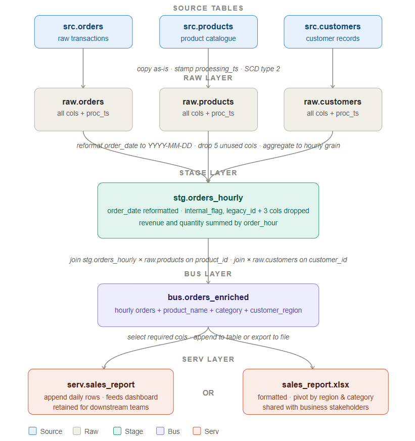
To make layer separation concrete, let’s walk through a real pipeline scenario. We have three source tables — src.orders, src.products, and src.customers — and our goal is to produce a hourly sales report that feeds a dashboard and can also be exported as an Excel file for business stakeholders. Here is how the data moves through each layer.
Source Tables
We start with three tables coming from upstream source systems:
src.orders contains raw transactional data — every order placed, with columns like order_id, customer_id, product_id, order_date, quantity, and revenue. This table also contains a number of internal system columns that are not relevant to our reporting use case.
src.products is a product catalogue that holds product_id, product_name, category, and pricing information.
src.customers holds customer records including customer_id, customer_name, region, and account tier.
These source tables are owned by upstream systems and we treat them as read-only. We never transform or write back to them.
Raw Layer — Copy Everything, Change Nothing
The first step is to land a full copy of each source table into the raw layer without applying any transformation. The raw tables are raw.orders, raw.products, and raw.customers.
The only thing we add is a processing_ts column — a timestamp that records exactly when the record was ingested. We also apply SCD Type 2 logic, which means we preserve every historical version of a record rather than overwriting it. If a product’s name changes or a customer moves to a new region, the old version is retained alongside the new one. This gives us a complete audit trail.
The raw layer exists for one critical reason: if a data issue is discovered weeks later — a corrupted value, a source system bug, an unexpected schema change — you can come back to the raw layer and see exactly what arrived and when. Without it, you are flying blind during incident investigation.
Stage Layer — Clean, Reshape, and Aggregate
Once data is safely landed in raw, the stage layer is where we begin shaping it for analysis. All three raw tables flow into this layer, and the primary output is a single table: stg.orders_hourly.
Three things happen here:
Date reformatting. The order_date column arrives from the source system in a non-standard format. In the stage layer we reformat it to YYYY-MM-DD so that it is consistent with every other date field across our platform and compatible with our BI tools.
Column dropping. The source orders table contains columns that were relevant to the operational system but have no meaning in our reporting context — things like internal_flag, legacy_id, and system_generated_ref. We drop these five columns at the stage layer. This keeps downstream tables lean and prevents consumers from accidentally using columns they do not understand.
Hourly aggregation. Rather than keeping one row per individual order, we aggregate the data to an hourly grain. Revenue is summed, quantity is summed, and distinct order counts are calculated — all grouped by order_hour. This is the required grain for the dashboard, and doing the aggregation here means we do not repeat this expensive computation in every downstream query.
The stage layer is also the right place to handle data quality checks. If a revenue value is negative or a required field is null, those records can be flagged or filtered here before they propagate further.
Bus Layer — Enrich by Joining Tables
The bus layer takes the clean, aggregated stage data and makes it richer by joining it with reference data. The output is a single wide table: bus.orders_enriched.
We join stg.orders_hourly with raw.products on product_id to bring in product_name and category. We also join with raw.customers on customer_id to bring in customer_region and account_tier.
The result is a denormalised table where every row contains not just the hourly sales figures but also the full context around what was sold and who bought it. Downstream consumers should not have to perform these joins themselves — the bus layer handles it once, correctly, in a centralised place.
The bus layer is also where more advanced enrichments can happen. If you need to merge in legend or lookup data, compute ML features, or produce intermediate aggregations that multiple downstream tables share, this is the layer for it. Think of it as a reusable library of well-processed, enriched assets that any part of your platform can draw from.
Serv Layer — Deliver to Consumers
The serv layer is the final stop and the only layer that external consumers interact with. From bus.orders_enriched, we select the columns that consumers actually need — dropping anything that is internal or intermediate — and deliver the data in one of two ways depending on the use case.
Option 1 — Append to serv.sales_report. If the consumer is a dashboard or another data team, we append the latest hourly rows into a persistent table called serv.sales_report. This table is the single source of truth for the sales dashboard. It is stable, well-documented, and its schema does not change without a proper release process.
Option 2 — Export to sales_report.xlsx. If the consumer is a business stakeholder who works in Excel, we format the data into a structured spreadsheet — typically with a pivot by region and category — and deliver it as a file. The bus layer already has all the enrichment needed, so this export is simply a formatting step rather than any additional transformation.
The serv layer represents a contract with your consumers. Whatever you put here should be production-quality, tested, and reliable. Internal intermediate tables, experimental views, and half-processed datasets should never appear in this layer.
Leave a Reply